Learning Objectives
By the end of this module students will:
- Understand how computers represent letters, numbers, and symbols
- Be able to identify different information types
- Appreciate the difference between binary and text file types
- Be able to identify different computer languages used on computers to develop applications and construct webpages
- Understand what a relational database is and the difference between an SQL and noSQL database
- Appreciate data websites and the concepts behind how an application programming interface (API) can be developed to access such sites
- Representing & Managing Digital Spectra
- Understand the formats for representing spectral data
- JCAMP-DX, AnIML, ANDI, NetCDF, CSV, Tab delimited (XY format)
- Where to obtain reliable spectral information
- AIST Spectral Database for Organic Compounds (SDBS)
- NIST Chemistry WebBook
- ChemSpider
- Simulated spectra
- Spectral software
- Understand the formats for representing spectral data
Table of Contents
This paper is broken into two parts, click on the title of each part to discuss it.
3.1 Chemical Property Data
Introduction
Chemical Informatics (CI), the application of information science to chemical data, is an interdisciplinary field of growing importance. The reason; there are lots of chemists, lots of chemicals, and chemists have lots of data about the chemicals. The result; it is increasingly more difficult to find the information you need, or even find out if the information you need exists, because the amount and global distribution of data is so vast. Scientists in the area of CI are therefore trying to find ways to identify, organize, characterize and integrate data from many different sources, stored in multiple ways using open and easily implemented techniques and technologies.
This module is focused on teaching you, a budding chemist, the basics behind information, how it’s stored, identified and manipulated – so that you can understand how to use it effectively and efficiently.
Basics of Computer Systems
For a course about chemical information we start at the lowest level – how computers deal with information internally. As a start, imagine you have a Word document that contains the following:
904-620-1938
Humans of course can very easily identify that this is a telephone number, but to a computer it looks like the following in its basic format – binary (more information on this later…)
00111001, 00110000, 00110100, 00101101,
00110110, 00110010, 00110000, 00101101,
00110001, 00111001, 00110011, 00111000
Whether it be on a regular hard disk drive (magnetic coating on a disk) or a flash/SSD (memory chips) all data on a computer is stored as 1’s and O’s (see http://www.pcmag.com/article2/0,2817,2404258,00.asp). As a result, all data on a computer must be represented in binary notation. Each recorded 1 or 0 is a ‘bit’ and eight bits make a ‘byte’. A byte is the basis of presenting data because eight bits, being either 1 or 0, can together represent numbers up to 255. This is because for each bit there are two possible permutations and eight bits gives 28 combinations - 256 values, or 0 thru 255.
In the early days of computer systems, a single byte was used as the way to represent text characters, and was defined by the American Standard Code for Information Interchange (ASCII – see http://www.ascii-code.com/). Initially, only the numbers 0-127 where used to represent letters, numbers, punctuation marks and symbols (32-127), and non-printed characters (0-31). Subsequently, extended ASCII was introduced which added accented characters, other punctuation marks, and symbols (128-255).
Looking back on the example of the telephone number above, we can now translate the binary into the telephone number
|
Binary |
Decimal |
ASCII Character |
|
00110000 |
48 |
‘0’ |
|
00110001 |
49 |
‘1’ |
|
00110010 |
50 |
‘2’ |
|
00110011 |
51 |
‘3’ |
|
00110100 |
52 |
‘4’ |
|
00110101 |
53 |
‘5’ |
|
00110110 |
54 |
‘6’ |
|
00110111 |
55 |
‘7’ |
|
00111000 |
56 |
‘8’ |
|
00111001 |
57 |
‘9’ |
|
00101101 |
45 |
‘-’ |
Although we still ‘use’ ASCII today, in reality we use something called UTF-8. This is easier to say than how it is derived - Universal Coded Character Set + Transformation Format - 8-bit. Unicode (see http://unicode.org) started in 1987 as an effort to create a universal character set that would encompass characters from all languages and defined 16-bits, two bytes -> 216 -> 256 x 256 = 65536 possible characters – or code points. Today, the first 65536 characters are considered the “Basic Multilingual Plane”, and in addition there are sixteen other planes for representing characters giving a total of 1,114,112 code points. Thankfully, we don’t need to worry because if something is UTF-8 encoded it is backward compatible with the first 128 ASCII characters.
It’s worth pointing out at this stage that the development of Unicode is a good thing for science. We speak our own language and have special symbols that we use in many different situations (how about the equilibrium symbol? ⇌ ) and so publishers in science and technology have developed fonts for reporting scientific research. Check out and install STIX fonts (http://www.stixfonts.org) which would not be possible without Unicode.
Information Data Types
Looking back at the telephone number in the previous section our identification of the characters is based off of two things – the fact that there are only digits and hyphens, and the pattern of digits and hyphens. Again though the computer knows nothing of this, it just knows that there is a string of 12 characters. So, in the context of humans representing information in computers it is not just important for us to use characters, we also need to know generically what they represent. This is critical to everything we do on a computer because we need to know how to process the characters.
In a broad sense characters represent either; text, numbers, or special formats. In the context of discussing the common ‘data types’ we are going to reference those that are used in the relational database software ‘MySQL’. More about what MySQL actually is later, for now we will look at the ways in which the program represents information that it stores (see http://dev.mysql.com/doc/refman/5.6/en/data-types.html for more details).
Numeric types
Representation of different numeric values is important because it is dependent on how they are used. Choosing the right type is critical to making sure there are no inconsistencies, especially when making comparisons or rounding in calculations.
- Integers – You would think that there is only one type of integer (i.e. an exact number), but it turns out that we have to think about how much space we use up storing the number on a computer not just its type. MySQL defines TINYINT, SMALLINT, MEDIUMINT, INT, and BIGINT. The definitions of these are based on how big the number is they can represent which in turn is based off how many bytes are used to store the number. For each of these (like all numeric values) you also have to specify if the first bit of the leading byte indicates ± or not.
- Fixed Point Numbers – DECIMAL (or NUMERIC) in MySQL are used to store values with a defined precision (a set number of decimal places) and thus are non-integer exact numbers. Using the syntax DECIMAL(X,Y) you can define a decimal with X total digits (max 65) and Y decimal digits (max 30), so DECIMAL(4,2) allows you to store from -99.99 through +99.99.
- Floating Point Numbers – Very important in computers, and chemistry, floating point numbers FLOAT and DOUBLE are used to represent non-exact decimal numbers that range from very small to very large. The difference between FLOAT and DOUBLE is FLOAT uses four bytes to store the number (accurate to seven decimal places) and DOUBLE uses eight bytes (accurate to 14 decimal places). FLOAT is normally good enough for scientific calculations as it can store -3.402823466E+38 to -1.175494351E-38 and 1.175494351E-38 to 3.402823466E+38. These definitions work with the common IEEE standard of floating point arithmetic (see https://dx.doi.org/10.1109%2FIEEESTD.2008.4610935)
String Types
The differences between string types is primarily based on how much space they take up and how easy they are to search. Thinking about the application of the string is important especially deciding if a string should be exclusive or inclusive. Also, realize that there are situations where you might want to store a number as a string.
- Fixed Length Strings – CHAR allows you to define a string of characters (up to 30) of an exact length. If the string length is lower than the number of characters it is padded with spaces after the text. TINYTEXT, TEXT, MEDIUMTEXT, and LONGTEXT store 255, 65,535, 16,777,215, and 4,294,967,296 characters respectively (no extra spaces).
- Variable Length Strings - VARCHAR allows you to define a string up to 65,535 characters in length – it therefore has a variable maximum length. No spaces are added.
- Predefined String Types – There are times where you want to store strings but not just anything. Take for example a field that stores the size of a shirt – small, medium, or large. Using ENUM (short for enumerated) you define the list of possible strings that the field can take. If you try and store any other value nothing gets stored. You can also expand this idea to use more than one value from a defined list using SET. You might recognize these string types as they are commonly used to populate dropdown menus and multiple select lists in web pages.
Other Types
There are many other types of information that are stored some common ones are
- Dates, Times and Timestamps – Common formats exist for representation of dates and exact points in time. These of course are just special format text strings that are standardized so that computers can interpret them (you can do the same for telephone numbers, social security numbers, etc.). DATE format is 'YYYY-MM-DD', TIME format is 'HH:MM:SS', and DATETIME is 'YYYY-MM-DD HH:MM:SS'. TIMESTAMP looks the same as DATETIME except it stores the data internal factoring in the local time zone using the Coordinated Universal Time (UTC) format (see http://www.cl.cam.ac.uk/~mgk25/iso-time.html)
- Boolean – True or False is stored as a TINYINT(1) where 1 is true and 0 is false
- Binary – Everything so far has be stored in character strings but there are situations where you might want to store byte strings – or binary. This is more technical than we need so we don’t have to worry about it. It is fun to point out though that Binary Large Objects (BLOBs) can be used to store binary files like images, audio, etc.
Common Computer Files and Formats
The mention of binary files in the previous sections highlights that there are differences in how data is stored by computers. Traditionally, programs or applications are stored in binary format because they contain code that is used to allow the program to run and thus should not be displayed as text (it’s not readable anyway). In addition, there are many non-text based files, images, audio, video etc. that need to store their content in a format that is efficient – a place where UTF-8 (ASCII) is not needed. Historically though the most important reason for applications and files being stored as binary is that it gave the developer a way to protect their work and make money off of it. If the application they have written stores the files in a proprietary format (one that only the application can read and write) then no one else can work with the file without licensing the software used to create it.
In the early years, without the presence of the Internet this model worked well. But once we all became connected and more and more armchair software developers started developing free software, a significant push back started with this model. People wanted to be able to share documents and not have to pay high licensing fees just to be able to read a letter they sent out to their relatives. Although a lot of progress has been made in making file formats open and based on community standards, there are still a lot of issues will proprietary file formats, especially in the sciences. If you think about it, any data you get off of an instrument is stored in a proprietary format – if you want to get the data into Microsoft Excel for instance you have to export it. In a lot of cases you are not getting all the information that was gathered – but more about that later.
Microsoft is a good example of a company that used a proprietary binary file format for saving documents from all its applications, that has transitioned to an open standard text based format. In 2000 Microsoft started producing versions of its files (starting with Excel) in what was to become the Open Office eXtensible Markup Language (OOXML), a standard released by ECMA in December 2006 (see http://www.ecma-international.org/publications/standards/Ecma-376.htm). XML is a text based markup language published by the World Wide Web consortium (http://www.w3.org/XML/) that is used to annotate text strings using tags. Hypertext Markup Language (HTML) used in web browsers is a limited version of XML primarily used for presentation.
Comparing the binary Word document format (.doc file) with the new OOXML (.docx file) format and plain text (.txt file) we can see the differences (available for download online).
The Word .doc File Format
The Word .docx File Format
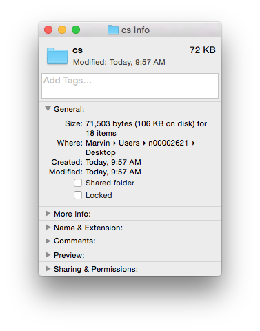
We see that the .doc file is unintelligible in a text reader and has over 22K characters – large considering the file contains only the text ‘Chemical Informatics’. The .docx file is also unreadable and slightly larger in size – but wasn’t this supposed to be in the OOXML text based format? It actually is, however the .docx file is actually a folder of XML files that is ZIP compressed into a single file. If you change the extension of a .docx file to .zip and un-compress it you see the folder of XML documents (that take up a lot of space – a problem with XML).
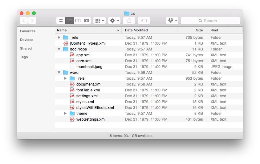
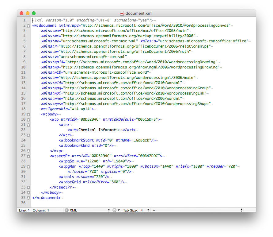
Finally, if you look inside the ‘document.xml’ file you find the text content. The other files in the folder are used to store information about the font used, the Word settings, the styles in use and an image of the file used by the operating system to display a thumbnail of the file content. The ‘document.xml’ contains the text of the file and other ‘markup’ – the XML – that provides the structure of the file, the layout of the page, and other important information
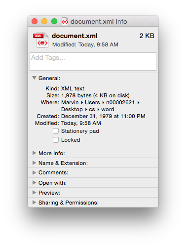
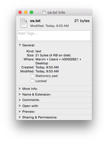
Of course if you just need the text (i.e. no formatting etc.) then you could use the .txt format. It’s got the same size 21 bytes, as the length of the text (including the carriage return as the end of the sentence). Sometimes less, is more…

Computer Languages for Information Science
While this class is not a course in programming, it is useful to know what it is out there that can be used to manipulate information, perform calculations, and organize data. As this is an introduction we will just touch on three that scientists/web developers use, but there are many more – each with different advantages. This discussion does not include the hard code application development platforms like C++, C#, etc.
Desktop Application (Windows, Mac) – Microsoft Excel
A lot of people think that Microsoft Excel is really for business people and not scientists. Certainly, Microsoft caters to the business community in terms of the table formats, graphics, and cell functions. Nonetheless, Excel has functionality that can be used in the context of informatics and, as you will see later in the course, can talk to webservers (websites) to retrieve data.
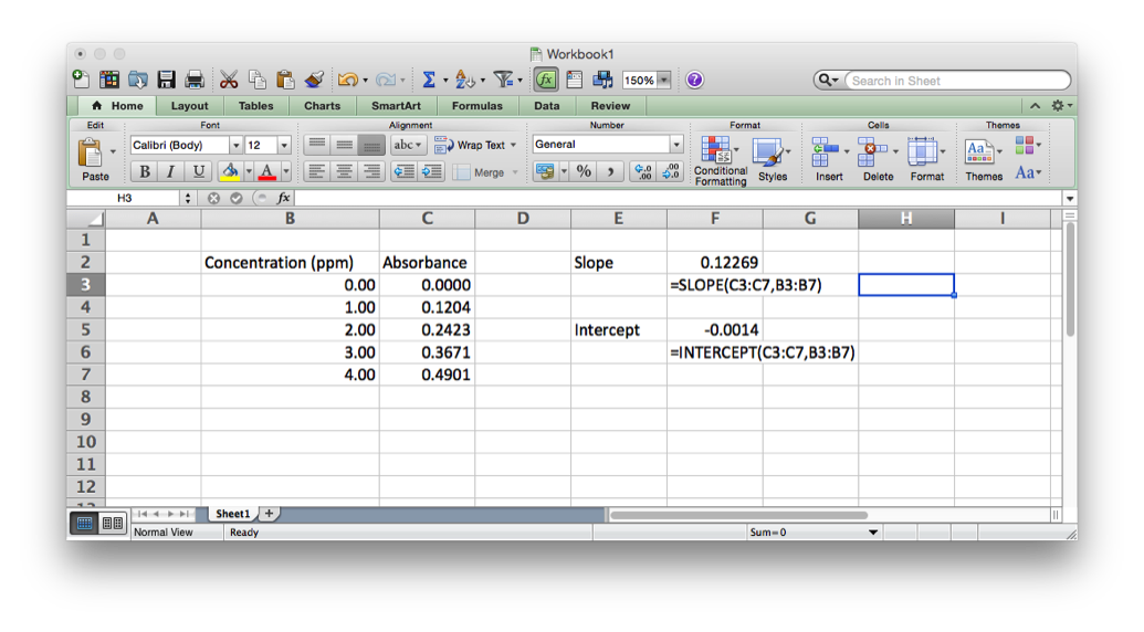
Excel has programming built-in in two ways. First, there are the in-cell functions. These are useful for text manipulation and basic math operations (see http://www.dummies.com/how-to/content/excel-formulas-and-functions-for-dummies-cheat-she.html). There are also some statistical functions like mean (AVERAGE), mode (MODE), median (MEDIAN) standard deviation (STDEV), as well as some more sophisticated functions related to linear regression (SLOPE and INTERCEPT).
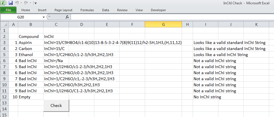
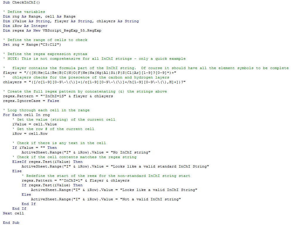
Then there is the much more sophisticated Visual Basic for Applications, (VBA), which sits behind Excel and is used to record the Macro’s run in Excel. VBA is much more a true programming language allowing for declaration of variables, loop structures, if-then-else conditionals and user defined functions. The script below is a quick example of how to check for strings to be a particular format – in this case the International Chemical Identifier, or InChI string (more later on this). This script tries to match the pattern that is defined to the text in each cell to tell if the string ‘looks’ like a valid InChI string. Whether it is would have to be tested in other ways…
Command Line Application (Any platform) – R
R (yes just the letter R) is a very popular statistical computing and graphics environment (see https://www.r-project.org/). R is sophisticated and extremely powerful so there is no way to show off its capabilities in a brief introduction, but to give you a flavor here are some things you can do. R is natively a command line application, so it does not have a graphical user interface (GUI) built-in that means it launches like other applications – you run it from the command line in the terminal. There are however many GUI’s for R – for example RStudio (https://www.rstudio.com).
In order to get data into R to do something with it you must either enter it or import it from a text file. If we look back at the linear regression example from Excel we see we have two arrays of data, the x data points (concentration) and the y data points (absorbance). If we wanted to enter these into R we would do it like this.
sh-3.2# R (run R)
> xpoints <- c(0.00,1.00,2.00,3.00,4.00)
> ypoints <- c(0.0000,0.1204,0.2423,0.3671,0.4901)
> lsfit(xpoints,ypoints)
$coefficients
Intercept X
-0.00140 0.12269
$residuals
[1] 0.00140 -0.00089 -0.00168 0.00043 0.00074
…
We enter the x and y data points as matrixes (you can also think of them as arrays) and then use them as inputs to the lsfit (least squares fit) function that is defined in R. It immediately spits out the slope, intercept and residuals (the differences between the y values and the calculated y values from the equation) as well as a lot of other details not shown above.
Browser Application (Any platform) – PHP
In the early days of the Internet every webpage you accessed was static, that is, it was a page of text in a file that had to be updated manually to change it. Today, the majority of websites are built using scripts that dynamically created the page when it is requested. This is because we expect sophistication (features), information (content), and immediacy (its up to date). Therefore, the web server needs to things to create the web pages: content (typically stored in a database – see the next section) and a scripting language that can logically build the page based on a set of commands. Current the most popular language to do this is called Pre-Hypertext Processor, or PHP (see http://php.net/).
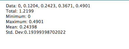
Just like R, it is impossible to show how capable PHP is in generating web pages on the fly, but a brief example script below shows how to calculate some statistics in a web page, with the output shown below it.
<?php
$data = [0.0000,0.1204,0.2423,0.3671,0.4901];
echo "Data: ".implode(", ",$data)."<br />";
echo "Total: ".array_sum($data)."<br />";
echo "Minimum: ".min($data)."<br />";
echo "Maximum: ".max($data)."<br />";
$mean=array_sum($data)/count($data);
echo "Mean: ".$mean."<br />";
$sumsquares=0;
foreach($data as $point) {
$sumsquares+=pow($point-$mean,2);
}
echo "Std. Dev: ".sqrt($sumsquares/(count($data)-1));
?>
Storing Information in Databases
A database is a system that stores information in a logical, organized format. Many applications on your computer (contacts, calendar, mail reader) rely on databases as the places to store the information that needs to be displayed in a way that allows the application to easily go grab the data.
While there are a number of styles of database the most common currently are relational. This means that data in different ‘tables’ is related together by the use of a unique id field, also called a foreign key. Each row of a table is given a unique value and this is then entered in a field in another table for any rows of data that are related to the information in the first table. Sounds complicated but it’s easy to see it in action in the upcoming examples.
Desktop Database
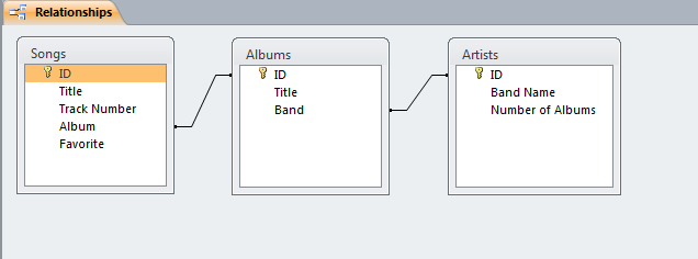
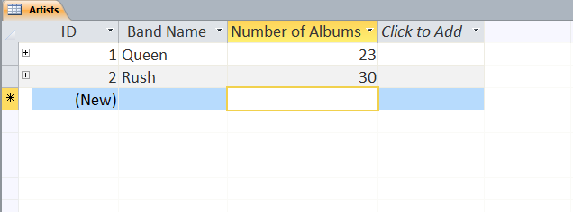
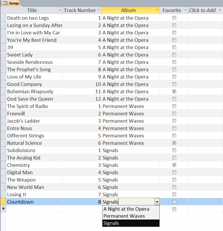
Microsoft Access has been a staple part of the Microsoft Office suite of applications since 1992. It often goes overlooked as there are a wider variety of uses for Word, Excel, and PowerPoint, but it is a powerful relational database that has found great use in business.
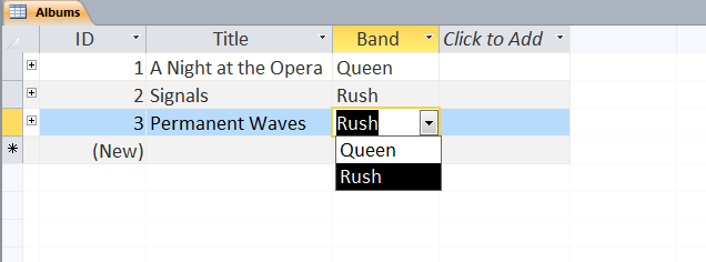
Users can define multiple tables of data (one entry is a row with multiple fields (columns)) and then link them together using unique ids that are automatically created on each row. Columns can be different data types (text, numeric, date/time, currency, etc.) or relational (lookup). The example below shows a small set of artists, albums, and songs that are related together via fields defined in the tables. The relationships can be see in the last image with the ‘Album’ field of the ‘Songs’ table being linked to the ID field of the ‘Albums’ table, and the ‘Band’ field of the ‘Albums’ table being linked to the ID field of the ‘Artists’ table. As can be seen in the figures, entering data in the linked fields is done through dropdown menu’s (to control what text is in the field) making it easier to create the table and providing the relationships.
Web-based Databases
Currently, the world of relational database is primarily geared toward the use of the Structured Query Language (SQL). SQL is a special programming language for retrieving data out of databases originally developed at IBM in the early 1970s. Relational Software (now called Oracle) created the first commercial software to implement SQL in the late 70s – called Oracle V2, and has subsequently become a major player in the database industry. Currently, there are many implementations of SQL databases, both commercial and open source (free), and most of them are accessible from scripting languages so they can be considered ‘Web-based’ databases.
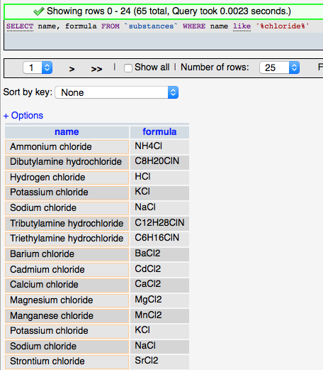
Although it grew out of the relational database model, SQL has deviated somewhat to include features and provide functionality needed for database applications. The basic structure of SQL is an English language sentence comprised of multiple parts using defined keywords. ‘SELECT’ is used to indicate that data is to be retrieved, ‘FROM’ is used to identify the table(s) from which the data is to be obtained, and ‘WHERE’ defines conditions on which the command searches. So the following SQL query (left) selects all the substance that have chloride (‘%' is used as a wildcard) in the their name and returns the names and formulas of those entries found (rather than all the fields (columns) in the substances table).
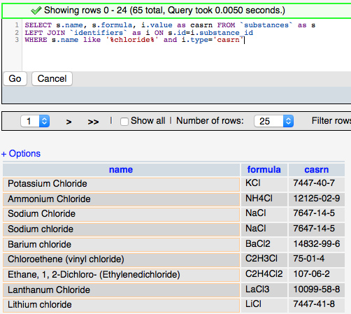
The more complicated query (right) adds the ‘JOIN’ syntax that is used to create relationships between tables on the fly so that related data can be retrieved in a single query. The designation LEFT JOIN means that all the data from the ‘LEFT’ (first) table is including in the results even if there is no related data in the ‘RIGHT’ (second) table. The keyword ‘AS’ is used to create an alias to a table to make the query shorter, and the keyword ‘ON’ is used to define the fields to join between the tables.
One current trend of note is the movement toward ‘NoSQL’ databases. This is somewhat of a misnomer as the class of databases this commonly refers to are really non-relational in nature and as a result there is no need to use SQL queries (although some do). The database model types lumped into the NoSQL classification are: Column, Document, Key-Value, Graph, and Multi-model based. Many of these have only been developed in the last few years as a response to interest in big data – applications where very fast processing of large (distributed) datasets is required. Graph based databases are of interest in many situations due to their lack of a data model and representation of ‘semantic’ data or subject-predicate-object triples. These databases have their own query language, SPARQL which is the interestingly recursive acronym that stands for ‘SPARQL Protocol and RDF Query Language’.
Accessing Data on Websites and Application Programming Interfaces (APIs)
To bring this module to a close it is important to discuss the ramifications of all that we have covered in the previous sections. By now you will hopefully have come to the realization that i) there is a lot of information/data in the world, ii) organizing it and identifying it is a important and huge undertaking, and iii) accessing chemistry related data in this environment cannot be done by a Google search. A lot of what chemical informatics is about is providing ways to deal with lots of data, describing best practices of how to identify and store information, and developing tools that allow scientists to find and retrieve quality information that can be used for teaching and research.
One of the fundamental parts of this is understanding where good chemistry data is, working out how to efficiently search it – based on chemical terms – and how to download it so that you can use it. In the previous sections you have seen examples of how data can be processed and stored in databases, but how do you get the data? It turns out that bringing SQL databases and scripting languages together to build webpages is only one facet of their usefulness. Increasingly websites are being built to serve up data, that is, they are designed to allow the user to search databases via well-defined standards and return the results for both human and computer use.
Over the last few years the design of websites that follow the Representational State Transfer (REST) paradigm have become popular as their design allows websites to become web services. What that means is if you know how to construct the URLs for pages on these websites you can anticipate the information that you are going to see on the page that is returned. This concept is so much easier to see in practice.
One website that has a large amount of chemical metadata (information about chemicals – not chemical data like melting points etc.) is the NIH Chemical Identifier Resolver (CIR) website (see http://cactus.nci.nih.gov/chemical/structure). The website allows you to get information by writing it in the general format below.
http://cactus.nci.nih.gov/chemical/structure/"structure identifier"/"representation"
In this context “Structure Identifier” means any of the following: chemical names, SMILES, InChI Strings and Keys, and NIH identifiers like FICTS and FICuS. What you get back from a search is determined by the “representation” part of the URL and includes all of those above and ‘sdf’ (otherwise known as MOL file), ‘formula’ and ‘image’. So, using the URL below:
http://cactus.nci.nih.gov/chemical/structure/arsinic acid/names
prints out the names of this compound that are in the CIR system – for humans to read. If you use a computer to access the site (i.e. via a scripting language like PHP) you can also request the data be sent to you as XML using.
http://cactus.nci.nih.gov/chemical/structure/arsinic acid/names/xml
which returns the following document.
<request string="arsinic acid" representation="names">
<data id="1" resolver="name_by_opsin" notation="arsinic acid">
<item id="1" classification="pubchem_iupac_name">arsinic acid</item>
<item id="2" classification="pubchem_substance_synonym">CHEBI:29840</item>
<item id="3" classification="pubchem_substance_synonym">HAsH2O2</item>
<item id="4" classification="pubchem_substance_synonym">[AsH2O(OH)]</item>
<item id="5" classification="pubchem_substance_synonym">arsinic acid</item>
<item id="6" classification="pubchem_substance_synonym">dihydridohydroxidooxidoarsenic</item>
</data>
</request>
This is useful because it contains additional information (metadata) about the type of name that an entry is and it makes it easy for a script to take the data and do something with it – like put it in another database.
There are many sites that chemists can use to get chemical data, ChemSpider (http://www.chemspider.com/), PubChem (https://pubchem.ncbi.nlm.nih.gov/), and the NIST Webbook (http://webbook.nist.gov/chemistry/). Each has a different set of data but all have a standard way to interact with their website. To encourage users to take full advantage of the search features many sites will publish the Application Programming Interface (API) that delineates what you can search for and how to do it. Facebook has an API, Twitter has an API, Instagram… the list goes on. API’s are the way in which websites can ‘’talk” to other websites to integrate data, or present ‘widgets’ that allow you to see what’s happening on one site when you are on another. A good example of a well documented and sophisticated API for chemistry data is the one at PubChem (see https://pubchem.ncbi.nlm.nih.gov/pug_rest/PUG_REST.html) which has a nice tutorial at https://pubchem.ncbi.nlm.nih.gov/pug_rest/PUG_REST_Tutorial.html. With over 94 million compounds to search you are sure to find something!
Chemical Property Data Assignment
Now that you know enough about computers and metadata to be information gurus here's an exercise to put your skills to the test. You will create an Excel spreadsheet of chemical property data and metadata.
1. Using the research skills you learned in module 1a find a web page that has a lot of chemical property data on it. It should not be a page that is part of an existing online database, rather a page that is maintained by a science professional(s) as a service to the community. It should also have the following attributes:
- Useful property data (with units as appropriate) and/or metadata (i.e. descriptors)
- Chemical names/formulas clear enough to be find CAS numbers and molecular weights
- Citation(s) indicating the source(s) of the data (i.e. its experimental data)
- Example pages that meet these criteria are:
2. Save the web page as a text file on your computer. Most browsers offer you the option to save as text. This removes any HTML formatting and makes it easier to work with the actual data.
3. Import that text file into Excel. Do this by opening Excel first and then opening the text from the file menu (see right). You should see the dialog box below. In most cases the 'delimited' option works best for importing data. You pick a character on the second dialog page to allow Excel to know how to put the data across different columns (tab, pipe (|), comma, etc.). This will help with organizing the data in the next step.

4.Organize the data that you have imported in columns (different data or metadata) and rows (compounds). Give a title to each column and underneath it identify the datatype for the column (text, enum, integer, float etc.). Some columns may be more than one datatype so try and pick the best one - i.e. the one that is most appropriate for all values that might logically be in that column. Include columns that contain the Chemical Abstracts Registry Number (CAS number) and molecular weights for all of the compounds in the table if they are not already part of the data. An example of what this might look like is below.

Table of Contents
- Log in to post comments
3.2 Representing and Managing Digital Spectra
#bottomRepresenting & Managing Digital Spectra
Since the early 1970’s microcomputers (as they were called at the time) have been a huge part of the development of scientific instrumentation. As computer control of instrumentation became more prevalent, there was a need to also interface the detectors of instruments to the computer so that data (analog or digital) could be captured as it was generated, rather than output it on oscilloscope screens or chart recorders (see https://en.wikipedia.org/wiki/Chart_recorder).
In the early years of the digital capture of spectral data the main limitation was storage capacity. As a result there was a practical limit on the time resolution (points per minute) and signal resolution (how many bits an analog signal was digitized as – see https://en.wikipedia.org/wiki/Analog-to-digital_converter). It wasn’t until the early 1980’s and the advent of the 5 1/4“ floppy disk which initially stored an amazing ~100 kB (0.1 MB) of data, that scientists were easily able to collect and save digital spectra.
Today, instruments generate a vast amount of data and file sizes can be up to several GB each for certain techniques (e.g. GC-MS). This module describes some of the common file formats for spectral data, websites where you can obtain reliable spectral data, and software for viewing/simulating spectra.
Spectral File Formats
As there are many instrument vendors, there are many different file formats for spectral data. This approach was supported vendors who developed the instruments and software to operate them; thus, in order to go back and view spectra you need to use their proprietary software – which of course gets updated on a regular basis and generates revenue. However, the majority of software does have an export format for the data (and maybe some of the spectral metadata) that can be directly imported into Excel or other applications because this has been a need for users for many years. This is typically as Tab-Delimited Text (.txt file) or Comma Separate Variable (.csv file) files.
Over time many scientists have lamented (even complained) that it would be much better if all of the data collected on instruments were stored in a common format that would make it easy to view and share data. While .txt and .csv files can be used for both activities, there has always been a need for a file format that supports both the spectral data and the associated metadata that describes the instrument type and settings, samples, analyte(s) and any other contextual information that gives the data value. Historically, this has been achieved using the following specifications (what are listed below are major specifications with formal standards – there are others that are less formally defined).
ANalytical Data Interchange (ANDI)
This is for mass spectrometry and chromatography data and is described by the ASTM Standards E1947 – Mass Spectrometry (http://www.astm.org/Standards/E1947.htm) and E1947 – Chromatography (http://www.astm.org/Standards/E1948.htm). ANDI uses the Network Common Data Form (NetCDF) self-describing data format that is generically defined to store array-oriented scientific data (http://www.unidata.ucar.edu/software/netcdf/).
Crystallographic Information Framework (CIF)
Used for crystallographic data only. This format is less traditional in its data organization than other formats because it not only contains x-ray crystallography patterns but a large, and very well organized, array of metadata about the system under study. This text format is a fundamental standard in the discipline of crystallography and authors of new crystallographic work must provide data in this format to get their work published. (http://www.iucr.org/resources/cif)
The Joint Committee on Atomic and Molecular Physical Data – Data Exchange format (JCAMP-DX)
For UV/Visible Spectrophotometry, Infrared, Mass Spectrometry, Nuclear Magnetic Resonance, and Electron Spin Resonance data. JCAMP-DX is currently administered by the International Union of Pure and Applied Chemistry (IUPAC) at http://www.jcamp-dx.org, although the format has not been actively updated in almost 10 years. Although JCAMP-DX has not formally been standardized, it is currently the de facto standard for sharing spectral data and all the major databases store their data in the format.
JCAMP-DX is a file specification consisting of a number of LABELLED-DATA-RECORDs or LDRs. These are defined to allow reporting of spectral metadata and raw/processed instrument data. The table below outlines some of the main LDRs in JCAMP-DX.
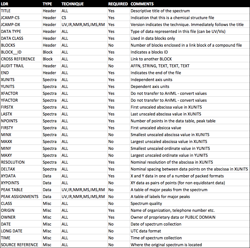
An example JCAMP-DX file is shown below.
##TITLE= Cholesterol (pktab1.jdx)
##JCAMP-DX= 5 $$home made
##DATA TYPE= MASS SPECTRUM
##DATA CLASS= PEAK TABLE
##ORIGIN= Dept of Chem, UWI, Mona, JAMAICA
##OWNER= public domain
##$URL= http://wwwchem.uwimona.edu.jm:1104/spectra/testdata/index.html
##SPECTROMETER/DATA SYSTEM= Finnigan
##INSTRUMENTAL PARAMETERS= LOW RESOLUTION
##.SPECTROMETER TYPE= TRAP
##.INLET= GC
##.IONIZATION MODE= EI+
##XUNITS= m/z
##YUNITS= relative abundance
##XFACTOR= 1
##YFACTOR= 1
##FIRSTX= 0
##LASTX= 386
##NPOINTS= 46
##FIRSTY= 0
##PEAK TABLE= (XY..XY)
0,0
41,520 43,1000 55,630 67,417 69,404 79,544 81,906 91,685 95,772 105,801
107,685 119,439 121,515 133,468 135,461 145,760 147,571 159,529 161,386
173,249 185,150 187,149 199,216 213,454 215,130 228,122 229,187 231,150
247,568 255,378 260,165 261,106 275,306 287,24 297,22 301,207 314,67
325,65 328,20 339,19 353,354 368,791 369,262 371,140 386,324
##END=
Note the LDRs for XFACTOR and YFACTOR. Although in the above example these LDRs are both 1 (because the raw data is already integers), these factors are commonly used to represent numeric values with a large number of decimal places as integers so that only one or two numbers (the factors) have to be stored as decimal values. This means that storage of rounded numbers is minimized and any error incurred because of rounding is applied evenly to all the data points. An example of data in this format is below.
##YFACTOR= 9.5367E-7
…
##XYDATA= (X++(Y..Y))
4400 68068800 68092800 68145600 68100800 68140800 68232000
4394 68304000 68316800 68195200 68152000 68182400 68176000
4388 68240000 68252800 68156800 68156800 68236800 68292800
4382 68302400 68265600 68233600 68214400 68224000 68284800
4376 68353600 68334400 68219200 68230400 68315200 68276800
4370 68259200 68264000 68257600 68316800 68292800 68339200
The data in a JCAMP-DX file can be all be compressed using a number of different human readable compression formats. This capability was added in order that spectral files were not to large for the storage media available (see above). There are four formats for compression, called ASCII Squeezed Difference Format (ASDF) outlined in one of the original articles on the JCAMP-DX format (http://old.iupac.org/jcamp/protocols/dxir01.pdf). These are listed below and use the letters as pseudo-digits.
|
Pseudo-digits for ASDF Formats |
|
|
1. ASCII digits |
0 1 2 3 4 5 6 7 8 9 |
|
2. Positive SQZ digits |
@ A B C D E F G H I |
|
3. Negative SQZ digits |
a b c d e f g h i |
|
4. Positive DIF digits |
% J K L M N O P Q R |
|
5. Negative DIF digits |
j k I m n o p q r |
|
6. Positive DUP digits |
S T U V W X Y Z s |
Note: The above characters replace the leading digit, sign, and preceding space for SQZ, DIF, and DUP forms.
The remaining digits of a multi-digit number are standard ASCII.
|
Simple Examples of ASDF Formats |
|
|
FIX Form: (22 chars) |
1 2 3 3 2 1 0 -1 -2 -3 |
|
PAC Form: (19 chars) or: |
1+2+3+3+2+1+0-1-2-3 1 2 3 3 2 1 0-1-2-3 |
|
SQZ Form: (10 chars) |
1BCCBA@abc |
|
DIF Form: (10 chars) |
1JJ%jjjjjj |
|
DIFDUP Form: (7 chars) |
1JT%jX |
As can be seen, the best compression is obtained by using the DIFDUP format which results in a 22/7 or 3.14x compression of the data. However, this is not always the amount of compression that will get because it depends on how variable the data points are in the file and it is important to choose the right format to get the best compression.
In addition to these existing formats there are a couple of newer formats that will eventually replace the JCAMP-DX specification.
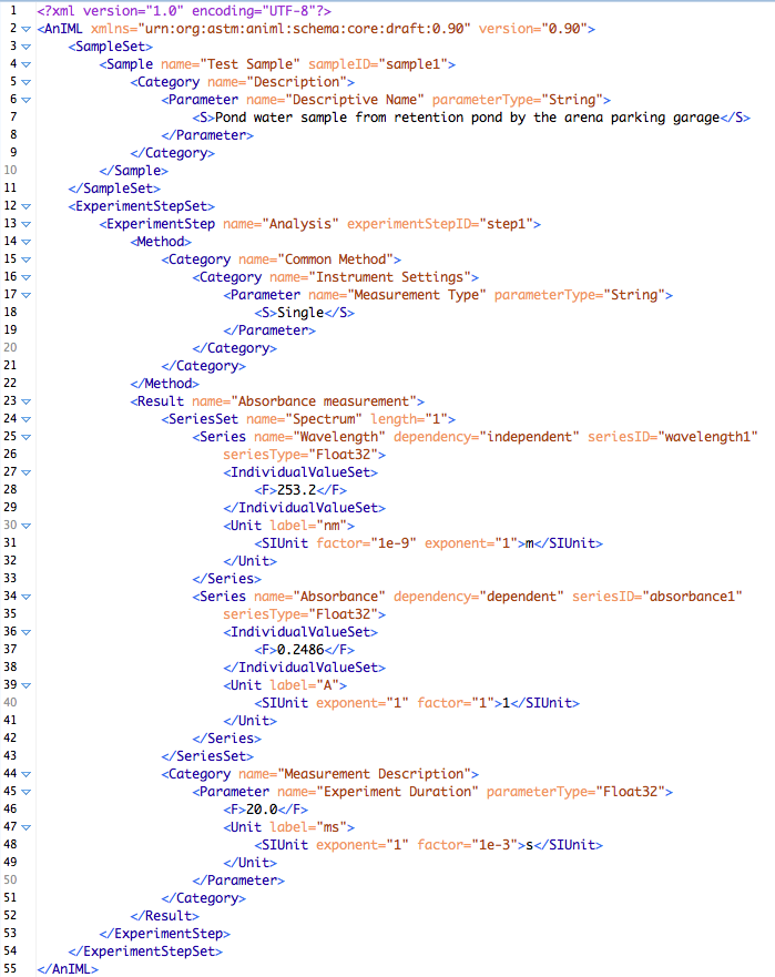
Analytical Information Markup Language (AnIML)
For all spectral data. AnIML is an eXtensible Markup Language (XML) format for storing instrument data and metadata under development since 2004 (http://animl.sourceforge.net). The specification is being coordinated under the American Standards and Testing of Materials (ASTM) E13.15 committee on analytical data.
It was recognized in 2004 that there needed to be a successor to JCAMP-DX because of i) advances in technology, ii) a recognized need to represent data from all analytical techniques, and iii) issues with variants of JCAMP-DX that made interoperability of the files difficult. AnIML files consist of up to four data sections; SampleSet, ExperimentStepSet, AuditTrailEntrySet, and SignatureSet. By design very little data/metadata is required so that legacy data, which may not have much or any metadata to describe it, can be stored in the AnIML format. An example ‘minimum’ AnIML file is shown below:
Allotrope Document Format
For all analytical data. The Allotrope Foundation was formed in 2012 from seven (now twelve) pharma companies around the notion of changing instrument data standards so that they were uniform across all instrument vendors. Three years later, Allotrope has just made available the first version of the Allotrope Document Format (ADF) that is based on the HD5 format for managing and storing data (https://www.hdfgroup.org/HDF5/). The ADF format stores data and metadata from the entire laboratory process (not just the instrument data) and is arrange in layers for metadata (using controlled vocabularies and ontologies), data, and linked files. The specification is so new that it has not yet been released to the community, but should be out by the end of the year. See http://www.allotrope.org.
Other spectral file formats
Lists of file formats for the following analytical techniques can be found at
- Mass Spectrometry - https://en.wikipedia.org/wiki/Mass_spectrometry_data_format
- NMR - https://en.wikipedia.org/wiki/Nuclear_magnetic_resonance_spectra_database
Sources of Spectral Data
AIST Spectral Database for Organic Compounds (SDBS) - http://sdbs.db.aist.go.jp
This database from Japan has a wealth of spectral information and is the best for searching, as there are many options to find what you need. Sadly, the majority of the spectra are presented as image files only (no JCAMP-DX) with only numeric peak data for MS and 1-NMR spectra (click the ‘peak data’ button. Currently, the site has the following amounts of spectral data:
- MS: ~25000 spectra
- 1H NMR: ~15900 spectra
- 13C NMR: ~14200 spectra
- FT-IR: ~54100 spectra
- Raman: ~3500 spectra
- ESR: ~2000 spectra
NIST Chemistry Webbook - http://webbook.nist.gov/chemistry/
The NIST Webbook is a prime source of spectral information about small organic compounds available as JCAMP-DX files, Scalable Vector Graphic (SVG - http://www.w3.org/Graphics/SVG/) files (an image format specified in XML), png image files, and scans of the original data (some from the 1960s). Searching for spectra on the site is done via the compound search and selection of the spectral data to be returned (if it is available for the compound(s) found). Other information such as thermodynamic property data, gas chromatograms (linked to original journal papers), and vibrational and electronic energy levels is also available on the site. Currently, the site has the following of spectral data:
- IR spectra for over 16,000 compounds
- Mass spectra for over 33,000 compounds
- UV/Vis spectra for over 1600 compounds
ChemSpider - http://www.chemspider.com
ChemSpider has over 10,000 spectra associated with chemical compounds in its database. Some of these are from commercial companies and organizations, but a large number have been uploaded by users of the website. As a result there may be spectra for compounds that are not available elsewhere. Finding compounds that have spectra available is not easy to do and in fact you can only access this information via one of the sites API’s (see below), which you need to create an account (free) to use. Access the following URL to get an XML file that lists all current spectral data by entering your security token in the ‘token’ field, which can be found on the http://www.chemspider.com/UserProfile.aspx page once you login on the ChemSpider website.
http://www.chemspider.com/Spectra.asmx?op=GetAllSpectraInfo
You can also search for spectra using the other commands on the http://www.chemspider.com/Spectra.asmx page, and search the mass spectra using commands found in the MassSpecAPI page at http://www.chemspider.com/MassSpecAPI.asmx. For example to search for peaks in a mass spectrum of mass 1000 ± 0.1 you can go to (no token required):
http://www.chemspider.com/MassSpecAPI.asmx/SearchByMass2?mass=1000&range=0.1
Other Sources of Spectra
- NIST Atomic Spectra Database - http://www.nist.gov/pml/data/asd.cfm
- NIST Molecular Spectra Databases - http://www.nist.gov/pml/data/molspec.cfm
- NMR Shift DB - http://nmrshiftdb.nmr.uni-koeln.de/
- Human Metabolome Database - http://www.hmdb.ca
- EPA Emissions Measurement Center Spectral Database -http://www3.epa.gov/ttn/emc/ftir/index.html
- MassBank - http://www.massbank.jp/
- Romanian Database of Raman Spectroscopy - http://rdrs.uaic.ro/index.html
Software
Spectral Viewers
- Jmol with JSpecView - http://jmol.sourceforge.net/ - the best and most widely used online and offline spectral viewer. Browser plugin provides a lot of features for display of data and export in different formats (right mouse click the plugin to see options for viewing spectra and exporting data). Go to the links below to test out the functionality
http://chemapps.stolaf.edu/jmol/jsmol/jsv.htm - drag and drop spectra viewing or search for molecules and display simulated spectra
http://chemapps.stolaf.edu/jmol/jsmol/jsv_jme.htm - draw a molecule and get simulated
spectrum
http://chemapps.stolaf.edu/jmol/jsmol/jsv_predict2.htm - same as the previous page but with 3D representation of molecular structure
- JCAMP Viewer - http://pslc.uwsp.edu/Viewers.shtml - web page looks old but software has been updated recently
- Flot JCAMP Viewer - http://webbook.nist.gov/chemistry - get from any page with spectra – requires web server
- SpeckTackle Javascript Viewer - https://bitbucket.org/sbeisken/specktackle - new on the scene – requires web server
- OpenSpectralWorks - http://scanedit.sourceforge.net/
- SpekWin32 - http://effemm2.de/spekwin/index_en.html
- OpenChrom - https://www.openchrom.net/ - primarily for chromatographic data but good for mas spectrometry as well
- ACD/Labs NMR Processor - http://www.acdlabs.com/resources/freeware/nmr_proc/index.php - NMR Only
- MestreLabs MNova - http://mestrelab.com/software/mnova/ - NMR Only ($)
- ChemDoodle - https://www.chemdoodle.com/ - reads all JCAMP files ($)
Spectral Prediction
- nmrdb.org - http://www.nmrdb.org/
- NMR Shift DB Online - http://nmrshiftdb.nmr.uni-koeln.de/nmrshiftdb/
- ChemDoodle - https://web.chemdoodle.com/demos/simulate-nmr-and-ms/
- ACD/Labs iLabs - https://ilab.acdlabs.com/iLab2/ (limited online trial)
Spectral Assignment
- Go to the NIST WebBook and download the following spectra in JCAMP-DX format
- Mass spectra for each of the three isomers of nitrobenzoic acid
- Gas phase IR spectra for each of the three isomers of nitroaniline
- Go to ChemSpider and download the HNMR spectra of the three isomers of xylene in JCAMP-DX (can you find them?)
- Go to the first JSpecView page above or download the JCAMP Viewer software for your OS. Import each of the spectra into the viewer you choose and export them to X,Y format.
- Finally, import each of the X,Y data files into Excel with one sheet for the MS data, one sheet for the IR data, and another sheet for the NMR data. Plot the three IR spectra on one graph (so they are overlaid) and do the same for the MS and NMR data (so you end up with three graphs). Save the file.
- Write a short paragraph comparing/contrasting for each of the three plots of overlaid IR, MS, and NMR spectra.
Table of Contents
- Log in to post comments
Comments 22
Unable to make hypothes.is annotation for 3.1
" What you get back from a search is determined by the “representation” part of the URL and includes all of those above and ‘sdf’ (otherwise known as MOL file), ‘formula’ and ‘image’. So, using the URL below:
http://cactus.nci.nih.gov/chemical/structure/arsinic acid/names
prints out the names of this compound that are in the CIR system – for humans to read. If you use a computer to access the site (i.e. via a scripting language like PHP) you can also request the data be sent to you as XML using."
Here's my question since I'm unable to make an annotation in hypothes.is as part of this assignment:
Are there any other representations that can be searched for which are not listed here? Also, what is an XML?
What is XML...
I don't know enough about hypothes.is to help so hopefully Dr. Belford will reply.
As for XML it stands for Extensible Markup Language and has been around since the mid 1990's. The importance of XML cannot be understated as a format to organize and annotate information. XML is very similar to HTML in that it uses 'tags' to identify the meaning of information i.e. '
904-620-1938 ' although HTML has only a finite set of tags whereas in XML they can be almost anything. If you read later on in this module Word's .docx file format is XML and many websites including the CIR one you mention can send the data as XML rather than HTML. For more general info about XML you can go to https://www.w3schools.com/xml/xml_whatis.asp.
Binary
This may just be a simple typo or I am misreading it, but I think the binary example used in the beginning for the phone number is for 904-620-1138 instead of 904-620-1938.
Oops
You are correct! I could claim that this a deliberate typo to see if students are reading the material, but in fact that's not true. I will fix it right away. Thanks for reporting it...
Stuart
Problem with Module 3 Assignment
The link for Thermodynamic Properties of Pure Substances in the first assignment seems not working. I keep having Page not Found report. Thanks
Phuc
bad link
Well, there's a lesson for you! :)
That professional has moved on, and their site has been cleared. Alas! This is the future for all web pages.
It was just an example, though. Best to ignore it.
Revised link
I have replaced the 'bad link' with one that is good for now. I also checked the WayBack Machine (http://archive.org/web/) for a copy of the page but its not there because the page was identified as protected by the institution.
Sorry, I did not pick this up earlier.
Importing MS data
Hi,
While working with JSpecView and JCAMP Viewer software, i tried importing the MS data of some compounds into Excel. For some reason it can't be save as a JDX (X,Y data file) in order to import it and use the data for a plot. How can i go about doing that? Thanks
Importing MS data
Many early MS data files only contained the largest 8 or so peaks and were not continuous data files.
You would need to plot these as bar charts or similar not as XY plots...
The JCAMP-DX files would have a label of ##XYPOINTS or ##PEAK TABLE= (XY..XY) and not ##XYDATA=(X++(Y..Y))
good project!
A nice student project would be to write a web page that lets the user paste in a set of XY data and then displays it in JSpecView and also creates a JDX file. Quite doable! :)
JCamp Error HNMR Files
I am trying to open a jdx file of one of the isomers of xylene to see NMR data, see url below for link to file. But Jcamp viewer for Windows throughs an error while reading the file. I have opened the same jdx file with programs online. So I am wondering if the Jcamp viewer for Windows updated on Feb. 23, 2017 is limited in specific types of data it can open/ versions of jdx files. I was able to open mass spec and IR jdx files with Jcamp viewer on my computer.
http://wwwchem.uwimona.edu.jm/spectra/xylonmr.jdx
Thanks
I have not been able to get
I have not been able to get the Windows JCamp viewer to work, either. Maybe it only works with spectra from their own machine.
JCAMP-DX Error HNMR Files - not for me
I just checked the o m p xylene NMR files and they all opened fine for me.
Maybe bad bandwidth?
Try saving to disk and checking you have the complete file ending with ##END=
I have the files downloaded
I have the files downloaded locally, and they appear complete (containing the '##END=' line). They still produce an error while opening.
JCAMP-DX Error HNMR Files - not for me
https://chemapps.stolaf.edu/nmr/viewspec2/
I was able to drag the file onto this page OK
InChi and commas in spreadsheet cells
Hi everyone,
My students posted a question to a sub TLO Google Sheet Connecting IUPAC name to PubChem but since nobody is "following" that thread (OLCCFac and OLCCstu are not following), I don't know if they will get an answer. I also cannot answer the question myself.
http://olcc.ccce.divched.org/comment/991#comment-991
The upshot of the post is that since inchi strings have commas in the data, the import treats that as new data and places it in a new cell. For example the inchi for hexane is InChI=1S/C6H14/c1-3-5-6-4-2/h3-6H2,1-2H3 and the 1-2H3 gets placed in a new cell.
I have taken a screen shot with the importdata line and placed that below. I am guessing there must be a precursor to add before the IMPORTDATA statement that should treat the returned data as a string variable. I just don't know what that would be. I do think that this is an interesting question as comma separated data will have this issue as spreadsheets interpret the commas as comma separated values. I tried to use =T(IMPORTDATA("http://opsin.ch.cam.ac.uk/opsin/"&A2&".inchi")) to convert it to text, but it still truncates to the first comma.
sample spreadsheet
If anyone wants to see it in action, I have provided a link to a copy of the spreadsheet. You can see that hexane has one column extra and 1,2-dichlorobutane has two columns extra.
https://docs.google.com/spreadsheets/d/1NqjX8B2D3OefnzBd5_FNuEyEmPWIv_CCFRz3cqsGASU/copy
InChi and Commas in Google Sheets
I agree with Bob on InChIKey, but sometimes you really just want the InChI. Also problems like this just bug the heck out of me, and I just know there's a solution! So, I think the following will work - Resolver an OPSIN.
=REGEXREPLACE(ArrayFormula(concatenate(IMPORTDATA("http://opsin.ch.cam.ac.uk/opsin/"&A2&".stdinchi")&",")), "\,\z", "")
=REGEXREPLACE(ArrayFormula(concatenate(IMPORTDATA("https://cactus.nci.nih.gov/chemical/structure/"&A2&"/stdinchi")&",")), "\,\z", "")
Otis
Add a second argument to IMPORTDATA
A simple solution is to add "\t" as a second argument to the IMPORTDATA function.
=IMPORTDATA("http://opsin.ch.cam.ac.uk/opsin/"&A2&".inchi","\t")
See it in action here: https://docs.google.com/spreadsheets/d/1YQpQiPgYJvfuHE5Tm6DMVw5hzwk3Cz0jByBp6eNwGeo/copy
simple solutions
Looks like we now have two solutions from Otis and Jordi. I think adding the\t is a little simpler. Where did you find the \t solution, and more importantly, what is the \t modifer doing? I am assuming it is a modifer for the IMPORTDATA statement that tells the IMPORTDATA to treat the data as a text string. I just couldn't find anything that suggested the modification. If you have a link to the modifications for IMPORTDATA, could you post it?
Thank you!
It is an undocumented feature...
Hi Ehren,
As far as I know this second argument is undocumented. It refers to the character used as column separator where "\t" means a tab character. Try using any other character instead.
This second argument is common in similar functions in Goggle Sheets and other systems, i.e SPLIT function.
Cheers,
Jordi
This is a normal/expected behavior of IMPORTDATA
Hi, all.
Actually it is an expected behavior of IMPORTDATA. It imports data from a given URL in a .csv (comma-separated values) or .tsv (tab-separated values) format. (Please see this document) As we know, InChI contains many commas, so the IMPORTDATA fuction interprets it as an array of values separated by commas. This is not a bug, but an expected behavior of the function.
Other line notations like SMILES and InChIKeys are not likely to have this issue because they don't use commas. However, I do expect the same problem if you try to get systematic chemical names (which use commas a lot) through IMPORTDATA function. And the same for any cases in which you expect any commas in imported data.
The solution suggest by Jordi essentially changes the expected output format from .csv to .tsv, so the commas are not interpreted as a field separator.